Planning images
Adding planning images
Each plan is associated with one or more planning images. These are added in the ![]()
Images tab of the plan developer dialog by selecting the Add New button. Images must be in NIFTI format, and are assigned a Label and a Modality. Any number of images useful for creating the plan may be added.
k-Plan doesn't support loading planning images in DICOM format. DICOM image stacks can be converted into NIFTI images using freely available converter tools like dcm2niix. For Windows users, a GUI based interface to dcm2niix is part of the freely available MRIcroGL viewer.
Primary planning image
One image must be designated as the primary planning image by selecting the corresponding checkbox when adding or editing the image. By default, this checkbox is automatically selected the first time an image is added. The Planning tab is only enabled after the primary planning image is added.
The primary planning image defines the origin of the k-Plan world coordinate system, and is used to derive the acoustic and thermal material properties for the simulation. This image must be a computed tomography (CT) image, or an MR image that has already been converted to a pseudo-CT image.
It is essential that a high-quality primary planning image is used that:
- Captures the field of view (generally the complete head above the foramen magnum)
- Has sufficient resolution (using an in-plane resolution and slice thickness of less than 1 mm)
- Accurately captures the thickness and density variation of the skull bone
- Is free from artifacts (including artifacts from dental fillings or metal implants)
Optionally, any number of additional images may be added, for example, to help localise the target of interest. However, only the primary planning image is used by k-Plan to evaluate the plan.
Deleting the primary planning image
If the primary planning image for a particular plan is deleted, the position of the transducer and all sonications are also removed. This is because the primary planning image defines the world coordinate system, and the transducer and target positions are defined in world coordinates.
CT calibration
To allow an accurate conversion of CT Hounsfield units (HU) to mass density, a calibration of the CT scanner should be performed using the same acquisition protocol used for the study. This is required because the HU in the image can vary depending on the CT acquisition settings.
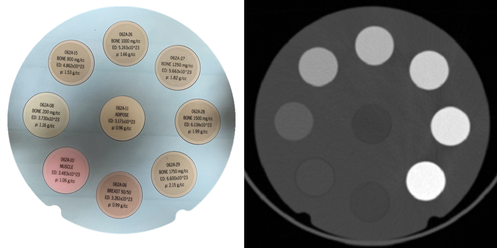
The calibration can be obtained using any suitable phantom with features that have varying (and known) mass density across the 1000 to 2200 kg/m3 range. The image below shows an example using a CIRS electron density phantom.
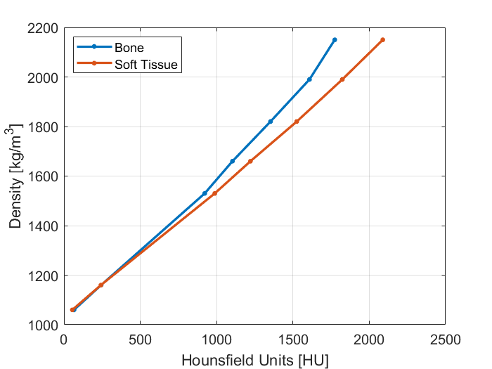
In general, the calibration does not depend strongly on tube current, but does depend on tube voltage and convolution kernel. To account for this, you should acquire a calibration image using each acquisition protocol and scanner you intend to use. The example below shows the difference in the calibration curves using bone and soft tissue convolution kernels for one particular CT vendor.
The CT calibration is defined as a piecewise linear mapping between radiodensity and mass density. The mapping is stored in a HDF5 file stored with a .kct extension. This must contain a 1 x N x 2 dataset called ct_calibration stored in single-precision in the root group. This dataset defines N radiodensity values in HU along with the corresponding mass density in kg/m3.
HDF5 files can be generated using most programming languages. The code snippet below shows how this file can be created using MATLAB. This example creates the default calibration. Note, the file creation from MATLAB automatically converts from column-major to row-major order such that the generated dataset has the correct dimensions.
MATLAB code to create CT calibration file
% define piece-wise linear mapping between HU and mass density in kg/m^3
hounsfieldUnits = [-990, 60, 1000, 1950];
massDensity = [1.2, 1060, 1530, 2150];
calibration = [hounsfieldUnits; massDensity];

% save calibration to HDF5 file
[I, J, K] = size(calibration);
filename = 'ct-calibration.kct';
h5create(filename, '/ct_calibration', [I, J, K], 'DataType', 'single');
h5write(filename, '/ct_calibration', single(calibration));

% set required file attributes
h5writeatt(filename, '/', 'application_name', 'k-Plan', 'TextEncoding', 'system');
h5writeatt(filename, '/', 'file_type', 'k-Plan CT Calibration', 'TextEncoding', 'system');
Please contact your k-Plan distributor if you do not have a suitable phantom and would like to arrange to have one shipped to you, or if you have acquired a calibration image and need assistance with generating the corresponding CT calibration file.
Default CT calibration
If no calibration file is selected, k-Plan uses the default calibration defined in the code snippet above. These values were derived using an approximate average of the calibration curves acquired using calibration images from several different CT vendors. However, this should be used with caution, as the default calibration may not match the true calibration for the scanner and acquisition settings used.
Incorrectly scaled CT images
A small subset of CT images use a different normalisation that maps air to 0 HU and water to 1000 HU (instead of air to -1000 HU and water to 0 HU). These images will not be converted correctly using the default calibration.
Using MR as the primary planning image
Currently, it is not possible to directly use MR images as the primary planning image in k-Plan. However, MR images converted to pseudo-CT images can be used in place of a CT. Be aware that the quality of the derived pseudo-CT will directly affect the accuracy of the k-Plan simulation.
The generation of pseudo-CT images from MR images is an area of active research. Methods include: (1) segmenting an MR image and then applying book values for the Hounsfield units, (2) using deep learning models to generate a pseudo-CT from a T1-weighted MR image, and (3) directly mapping from specialised MR sequences that show increased bone contrast, such as UTE, ZTE, and PETRA.
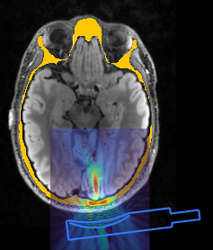
As an example, the image below shows a k-Plan simulation using a pseudo-CT created from the skin and skull masks generated using SimNIBS. The skull mask is shown as the yellow overlay.
If using a pseudo-CT image, then a CT calibration file should still be used. For deep-learning models, this should be acquired using the same CT scanner and acquisition protocols as the CT images used in the training set. This is because deep-learning models will generate images with similar characteristics to the images they are trained with. Similarly, if directly mapping from an MR image to a pseudo-CT image or assigning book values to a segmentation, the CT calibration file should be based on the CT images or properties used to derived the mapping curve.
MNI template
For running template simulations, CT and T1w MR images in MNI152 standard-space can be automatically loaded by selecting Add MNI Template.
The specific MR template used in k-Plan is the ICBM 152 2009c Nonlinear Symmetric 1×1x1mm template (mni_icbm152_t1_tal_nlin_sym_09c.nii) described in Fonov, V., Evans, A. C., Botteron, K., Almli, C. R., McKinstry, R. C., Collins, D. L., & Brain Development Cooperative Group. (2011). Unbiased average age-appropriate atlases for pediatric studies. Neuroimage, 54(1), 313-327.
The specific CT template used in k-Plan is described in Rorden, C., Bonilha, L., Fridriksson, J., Bender, B., & Karnath, H. O. (2012). Age-specific CT and MRI templates for spatial normalization. Neuroimage, 61(4), 957-965. The version included k-Plan has been padded to match the voxel dimensions of the MR template image.
Additional images (e.g., T2, segmentations, etc) registered to this template are available from the NIST-Lab website. See third party software for license details for both images.
When selecting Add MNI Template, the template CT image is loaded with a custom CT calibration curve. This maps the histogram of the template skull intensities to the average skull mass density values from the CT dataset described here.
MNI Coordinates
k-Plan does not work directly with MNI coordinates. To convert between [x, y, z] MNI coordinates and k-Plan world coordinates when working with the MNI template images, add [96, 132, 78] mm to the MNI coordinates in mm.
Image display settings
By default, a list of loaded images is displayed in a table on the right hand side of the ![]()
Planning tab of the plan developer dialog. The visibility of the images table can be toggled using the ![]() button.
button.
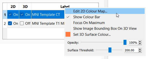
The order in which the images are rendered can be adjusted by dragging the numbers in the table up and down. In the example above, MNI Template CT is above MNI Template T1 MR in the table, so the CT image will be rendered on top of the MR image in the 2D views.
The visibility of each image in the 2D and 3D views can be changed by selecting the corresponding checkboxes. When the 3D checkbox is selected, an isosurface created using the specified Surface Threshold is displayed in the 3D view. Note, only the largest connected-component of the isosurface is displayed.
Additional settings for each image can be accessed by right-clicking on the image name:
- Edit 2D Colour Map: Opens the colour map dialog to allow the colour map and window/levels settings to be adjusted.
- Show Colour Bar: Displays a colour bar for the selected image on the 2D view.
- Focus On Maximum: Moves the position of the reslice cursor to the maximum value in the image.
- Show Image Bounding Box On 3D View: Shows a wire-frame outline of the image size on the 3D view.
- Set 3D Surface Colour: Sets the colour of the isosurface shown in the 3D view.
- Opacity: Sets the opacity of the image, where 0% is transparent, and 100% is opaque.
- Surface Threshold: Threshold used for the isosurface displayed in the 3D view.