Sonications
Adding a sonication
After the transducer has been positioned, one or more sonications can be added. For single-element and annular-array transducers, this action is performed by selecting the ![]()
Add Sonication For Current Transducer Position button in the Planning tab. For multi-element arrays, a sonication is added by selecting the ![]()
Add Sonication Target Using Alt-Click button, and then selecting the target position using Alt + Left Mouse Click on one of the 2D image views.
Sonication parameters
After a sonication is added, a new entry will be added to the sonication table. The visibility of the sonication table can be toggled using the ![]() button.
button.
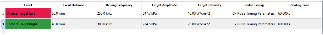
A number of parameters can be modified independently for each sonication. The visible parameters will depend on the type of transducer. To edit the parameters, click on the entry in the table.
- Label: Name used to identify the sonication. This name is prepended to the calculated field parameters so they can be identified in the image list, e.g.,
Cortical Target Left - Pressure. The same name is used to identify the sonication in the report. - Target Position: (Multi-Element Arrays Only) Position of the target in the k-Plan coordinate system.
-
Focal Distance: (Annular Arrays Only) Axial distance from the transducer to the focus in free-field. This distance can be specified in several ways:
- From the rear of the radiating surface of the transducer, or from a designated exit plane of the transducer.
- To the position of peak pressure, or to the centre of the -3 dB or -6 dB focal volume.
This distinction is specified in the transducer definition used by k-Plan (see the FDO and FD columns in the transducer library table), and can't be modified by the user. Generally, the distance aligns directly with the nomenclature used by the transducer manufacturer.
Parameter Limits
The transducer definition will typically also specify limits for the various sonication settings, for example, the minimum and maximum allowable focal distance. The sonication table will automatically enforce these limits.
-
Driving Frequency: The frequency used to drive the transducer.
-
Target Amplitude: The target amplitude specified as acoustic pressure. For single-element and annular array transducers, this sets the spatial-peak pressure in water (free-field). For multi-element arrays, this sets the in situ amplitude at the selected target location.
-
Target Intensity: The target amplitude specified as acoustic intensity.
Acoustic Intensity and Pressure
k-Plan primarily works with acoustic pressure, but the pulse-average acoustic intensity is also displayed as a derived parameter. This is calculated using \(I = \frac{p^2}{2Z}\), where \(p\) is the displayed pressure amplitude in Pa, \(I\) is the displayed acoustic intensity in W/m2, and \(Z\) is the characteristic acoustic impedance which is assumed to be \(1.5 \times 10^6\) Rayls.
-
Cooling Time: Additional time used for the thermal calculations to simulate the diffusion of heat from the sonicated tissue. The transducer is turned off during the cooling time. This can be useful to study the time taken for the tissue temperature to return to baseline. For linked sonications, this specifies the time between successive sonications.
Pulse timing parameters
The pulse timing parameters define the pulsing sequence used to drive the transducer. Note, these are used for the thermal simulations only. The acoustic simulations are performed independent of these parameters by running the model to steady state (the number of time steps is controlled by the grid traversals options in the Simulation Settings).
The pulse timing parameters can be modified by right-clicking on a sonication in the sonication table, and selecting Edit pulse timing parameters.... Dependent parameters (parameters automatically calculated from other parameters) are greyed out.
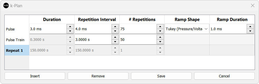
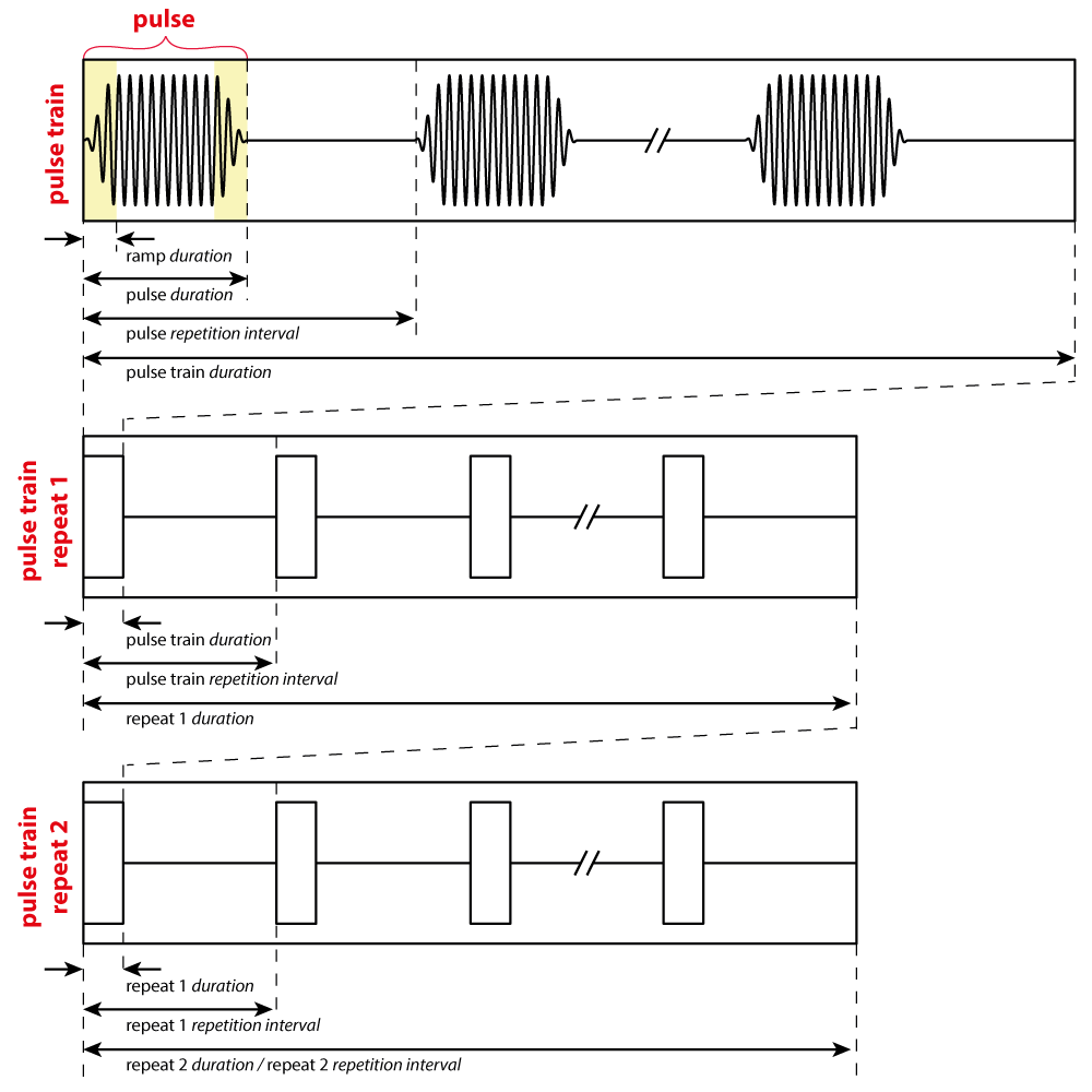
The pulse timing parameters are specified by nested levels of repeated pulses. Up to four levels are currently supported in k-Plan, and each has a unique name:
- Pulse
- Pulse Train
- Pulse Train Repeat 1 (or simply Repeat 1)
- Pulse Train Repeat 2 (or simply Repeat 2)
At each level, both the duration and repetition interval can be specified. Pulse levels can be added and removed by using the Insert and Remove buttons.
For the first level (pulse), a ramp can also be specified. The ramp shape is a Tukey window (raised-cosine) that varies smoothly from 0 to the maximum level over the specified ramp duration. The ramp duration is included in the pulse duration. For example, a 20 ms pulse duration with a 10 ms ramp duration creates a pulse that ramps up for 10 ms, then immediately ramps down for 10 ms. The ramp (Tukey-Window) can be applied to the voltage/pressure or to the power/intensity. If the ramp is applied to the voltage/pressure, the variation in the voltage/pressure will follow a Tukey window, and the variation in the power/intensity will follow the square of a Tukey window (and vice versa).
There are a number of restrictions which are enforced by the pulse timing table:
- The ramp duration cannot be more than half the pulse duration.
- The pulse train duration must be an integer multiple of the pulse repetition interval.
- The repeat 1 duration must be an integer multiple of the pulse train repetition interval (and so on).
-
At the last specified pulse level, the duration and repetition interval must be equal.
Single Pulse
To set a single continuous pulse, use only the
Pulselevel in the timing parameters table, and set theDurationequal to theRepetition Interval.